Accelerate data preparation using Amazon SageMaker Data Wrangler for diabetic patient readmission prediction

AWS Feed
Accelerate data preparation using Amazon SageMaker Data Wrangler for diabetic patient readmission prediction

Patient readmission to hospital after prior visits for the same disease results in an additional burden on healthcare providers, the health system, and patients. Machine learning (ML) models, if built and trained properly, can help understand reasons for readmission, and predict readmission accurately. ML could allow providers to create better treatment plans and care, which would translate to a reduction of both cost and mental stress for patients. However, ML is a complex technique that has been limiting organizations that don’t have the resources to recruit a team of data engineers and scientists to build ML workloads. In this post, we show you how to build an ML model based on the XGBoost algorithm to predict diabetic patient readmission easily and quickly with a graphical interface from Amazon SageMaker Data Wrangler.

Data Wrangler is an Amazon SageMaker Studio feature designed to allow you to explore and transform tabular data for ML use cases without coding. Data Wrangler is the fastest and easiest way to prepare data for ML. It gives you the ability to use a visual interface to access data and perform exploratory data analysis (EDA) and feature engineering. It also seamlessly operationalizes your data preparation steps by allowing you to export your data flow into Amazon SageMaker Pipelines, a Data Wrangler job, Python file, or Amazon SageMaker Feature Store.

Data Wrangler comes with over 300 built-in transforms and custom transformations using either Python, PySpark, or SparkSQL runtime. It also comes with built-in data analysis capabilities for charts (such as scatter plot or histogram) and time-saving model analysis capabilities such as feature importance, target leakage, and model explainability.

In this post, we explore the key capabilities of Data Wrangler using the UCI diabetic patient readmission dataset. We showcase how you can build ML data transformation steps without writing sophisticated coding, and how to create a model training, feature store, or ML pipeline with reproducibility for a diabetic patient readmission prediction use case.

We also have published a related GitHub project repo that includes the end-to-end ML workflow steps and relevant assets, including Jupyter notebooks.

We walk you through the following high-level steps:

• Studio prerequisites and input dataset setup
• Design your Data Wrangler flow file
• Create processing and training jobs for model building
• Host a trained model for real-time inference

Studio prerequisites and input dataset setup

To use Studio and Studio notebooks, you must complete the Studio onboarding process. Although you can choose from a few authentication methods, the simplest way to create a Studio domain is to follow the Quick start instructions. The Quick start uses the same default settings as the standard Studio setup. You can also choose to onboard using AWS Single Sign-On (AWS SSO) for authentication (see Onboard to Amazon SageMaker Studio Using AWS SSO).

Dataset

The patient readmission dataset captures 10 years (1999–2008) of clinical care at 130 US hospitals and integrated delivery networks. It includes over 50 features representing patient and hospital outcomes with about 100,000 observations.

You can start by downloading the public dataset and uploading it to an Amazon Simple Storage Service (Amazon S3) bucket. For demonstration purposes, we split the dataset into four tables based on feature categories: diabetic_data_hospital_visits.csv, diabetic_data_demographic.csv, diabetic_data_labs.csv, and diabetic_data_medication.csv. Review and run the code in datawrangler_workshop_pre_requisite.ipynb. If you leave everything at its default inside the notebook, the CSV files will be available in s3://sagemaker-${region}-${account_number}/sagemaker/demo-diabetic-datawrangler/.

Design your Data Wrangler flow file

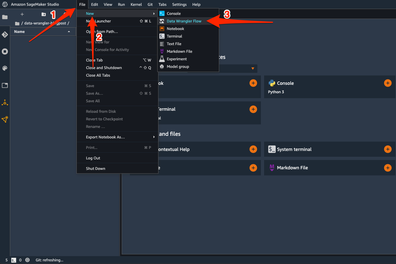
To get started – on the Studio File menu, choose New, and choose Data Wrangler Flow.

This launches a Data Wrangler instance and configures it with the Data Wrangler app. The process takes a few minutes to complete.

Load the data from Amazon S3 into Data Wrangler

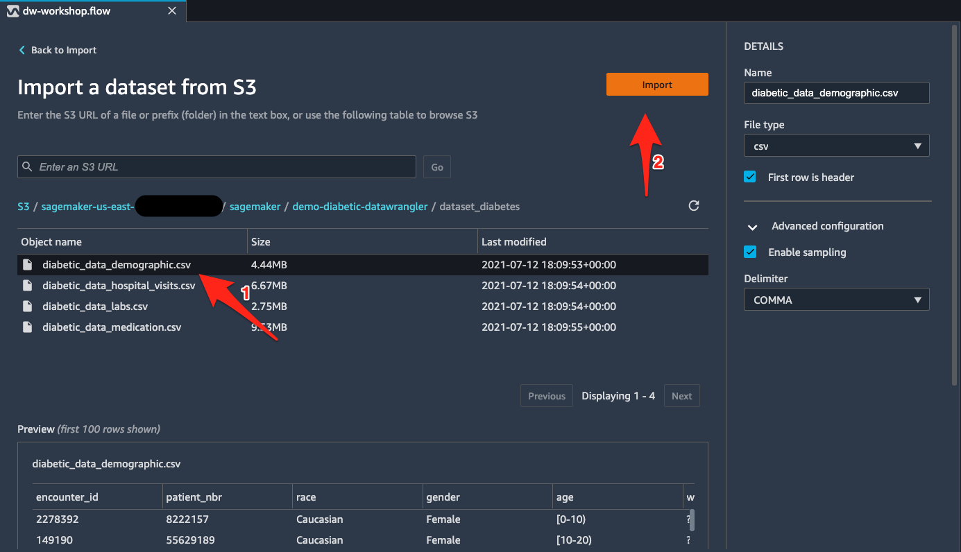
To load the data into Data Wrangler, complete the following steps:

1. On the Import tab, choose Amazon S3 as the data source.
2. Choose Add data source.
   

You could also import data from Amazon Athena, Amazon Redshift, or Snowflake. For more information about the currently supported import sources, see Import.

3. Select the CSV files from the bucket s3://sagemaker-${region}-${account_number}/sagemaker/demo-diabetic-datawrangler/ one at a time.
4. Choose Import for each file.

When the import is complete, data in an S3 bucket is available inside Data Wrangler for preprocessing.

Join the CSV files

Now that we have imported multiple CSV source dataset, let’s join them for a consolidated dataset.

1. On the Data flow tab, for Data types, choose the plus sign.
2. On the menu, choose Join.
   
3. Choose the diabetic_data_hospital_visits.csv dataset as the Right dataset.
4. Choose Configure to set up the join criteria.
   
5. For Name, enter a name for the join.
6. For Join type¸ choose a join type (for this post, Inner).
7. Choose the columns for Left and Right.
8. Choose Apply to preview the joined dataset.
9. Choose Add to add it to the data flow file.
   

Built-in analysis

Before we apply any transformations on the input source, let’s perform a quick analysis of the dataset. Data Wrangler provides several built-in analysis types, like histogram, scatter plot, target leakage, bias report, and quick model. For more information about analysis types, see Analyze and Visualize.

Target leakage

Target leakage occurs when information in an ML training dataset is strongly correlated with the target label, but isn’t available when the model is used for prediction. You might have a column in your dataset that serves as a proxy for the column you want to predict with your model. For classification tasks, Data Wrangler calculates the prediction quality metric of ROC-AUC, which is computed individually for each feature column via cross-validation to generate a target leakage report.

1. On the Data Flow tab, for Join, choose the plus sign.
2. Choose Add analysis.
   
3. For Analysis type, choose Target Leakage.
4. For Analysis name¸ enter a name.
5. For Max features, enter 50.
6. For Problem Type¸ choose classification.
7. For Target, choose readmitted.
8. Choose Preview to generate the report.
   

As shown in the preceding screenshot, there is no indication of target leakage in our input dataset. However, a few features like encounter_id_1, encounter_id_0, weight, and payer_code are marked as possibly redundant with 0.5 predictive ability of ROC. This means these features by themselves aren’t providing any useful information towards predicting the target. Before making the decision to drop these uninformative features, you should consider whether these could add value when used in tandem with other features. For our use case, we keep them as is and move to the next step.

9. Choose Save to save the analysis into your Data Wrangler data flow file.

Bias report

AI/ML systems are only as good as the data we put into them. ML-based systems are more accessible than ever before, and with the growth of adoption throughout various industries, further questions arise surrounding fairness and how it is ensured across these ML systems. Understanding how to detect and avoid bias in ML models is imperative and complex. With the built-in bias report in Data Wrangler, data scientists can quickly detect bias during the data preparation stage of the ML workflow. Bias report analysis uses Amazon SageMaker Clarify to perform bias analysis.

To generate a bias report, you must specify the target column that you want to predict and a facet or column that you want to inspect for potential biases. For example, we can generate a bias report on the gender feature for Female values to see whether there is any class imbalance.

1. On the Analysis tab, choose Create new analysis.
   
2. For Analysis type¸ choose Bias Report.
3. For Analysis name, enter a name.
4. For Select the column your model predicts, choose readmitted.
5. For Predicted value, enter NO.
6. For Column to analyze for bias, choose gender.
7. For Column value to analyze for bias, choose Female.
8. Leave remaining settings at their default.
9. Choose Check for bias to generate the bias report.
   

As shown in the bias report, there is no significant bias in our input dataset, which means the dataset has a fair amount of representation by gender. For our dataset, we can move forward with a hypothesis that there is no inherent bias in our dataset. However, based on your use case and dataset, you might want to run similar bias reporting on other features of your dataset to identify any potential bias. If any bias is detected, you can consider applying a suitable transformation to address that bias.

10. Choose Save to add this report to the data flow file.

Histogram

In this section, we use a histogram to gain insights into the target label patterns inside our input dataset.

1. On the Analysis tab, choose Create new analysis.
2. For Analysis type¸ choose Histogram.
3. For Analysis name¸ enter a name.
4. For X axis, choose readmitted.
5. For Color by, choose race.
6. For Facet by, choose gender.
7. Choose Preview to generate a histogram.
   

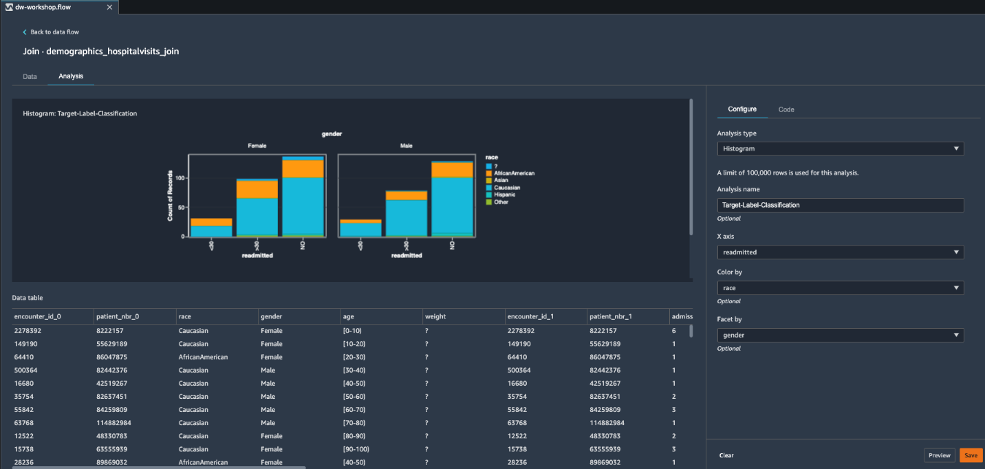
This ML problem is a multi-class classification problem. However, we can observe a major target class imbalance between patients readmitted <30 days, >30 days, and NO readmission. We can also see that these two classifications are proportionate across gender and race. To improve our potential model predictability, we can merge <30 and >30 into a single positive class. This merge of target label classification turns our ML problem into a binary classification. As we demonstrate in the next section, we can do this easily by adding respective transformations.

Transformations

When it comes to training an ML model for structured or tabular data, decision tree-based algorithms are considered best in class. This is due to their inherent technique of applying ensemble tree methods in order to boost weak learners using the gradient descent architecture.

For our medical source dataset, we use the SageMaker built-in XGBoost algorithm because it’s one of the most popular decision tree-based ensemble ML algorithms. The XGBoost algorithm can only accept numerical values as input, therefore as a prerequisite we must apply categorical feature transformations on our source dataset.

Data Wrangler comes with over 300 built-in transforms, which require no coding. Let’s use built-in transforms to apply a few key transformations and prepare our training dataset.

Handle missing values

To address missing values, complete the following steps:

1. Switch to Data tab to bring up all the built-in transforms
2. Expand Handle missing in the list of transforms.
3. For Transform, choose Impute.
4. For Column type¸ choose Numeric.
5. For Input column, choose diag_1.
6. For Imputing strategy, choose Mean.
7. By default, the operation is performed in-place, but you can provide an optional Output column name, which creates a new column with imputed values. For our blog we go with default in-place update.
8. Choose Preview to preview the results.
9. Choose Add to include this transformation step into the data flow file.
   
10. Repeat these steps for the diag_2 and diag_3 features and impute missing values.

Search and edit features with special characters

Because our source dataset has features with special characters, we need to clean them before training. Let’s use the search and edit transform.

1. Expand Search and edit in the list of transforms.
2. For Transform, choose Find and replace substring.
3. For Input column, choose race.
4. For Pattern, enter ?.
5. For Replacement string¸ choose Other.
6. Leave Output column blank for in-place replacements.
7. Choose Preview.
8. Choose Add to add the transform to your data flow.
   
9. Repeat the same steps for other features to replace weight and payer_code with 0 and medical_specialty with Other.
   

One-hot encoding for categorical features

To use one-hot encoding for categorical features, complete the following steps:

1. Expand Encode categorical in the list of transforms.
2. For Transform, choose One-hot encode.
3. For Input column, choose race.
4. For Output style, choose Columns.
5. Choose Preview.
6. Choose Add to add the change to the data flow.
   
7. Repeat these steps for age and medical_specialty_filler to one-hot encode those categorical features as well.

Ordinal encoding for categorical features

To use ordinal encoding for categorical features, complete the following steps:

1. Expand Encode categorical in the list of transforms.
2. For Transform, choose Ordinal encode.
3. For Input column, choose gender.
4. For Invalid handling strategy, choose Keep.
5. Choose Preview.
6. Choose Add to add the change to the data flow.
   

Custom transformations: Add new features to your dataset

If we decide to store our transformed features in Feature Store, a prerequisite is to insert the eventTime feature into the dataset. We can easily do that using a custom transformation.

1. Expand Custom Transform in the list of transforms.
2. Choose Python (Pandas) and enter the following line of code:

   # Table is available as variable `df`
   import time
   df['eventTime'] = time.time()

3. Choose Preview to view the results.
4. Choose Add to add the change to the data flow.
   

Transform the target Label

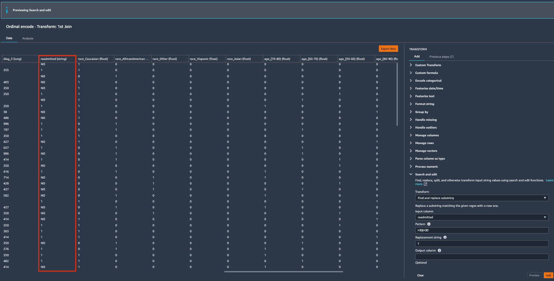
The target label readmitted has three classes: NO readmission, readmitted <30 days, and readmitted >30 days. We saw in our histogram analysis that there is a strong class imbalance because the majority of the patients didn’t readmit. We can combine the latter two classes into a positive class to denote the patients being readmitted, and turn the classification problem into a binary case instead of multi-class. Let’s use the search and edit transform to convert string values to binary values.

1. Expand Search and edit in the list of transforms.
2. For Transform, choose Find and replace substring.
3. For Input column, choose readmitted.
4. For Pattern, enter >30|<30.
5. For the Replacement string, enter 1.

This converts all the values that have either >30 or <30 values to 1.

6. Choose Preview to view the results.
7. Choose Add to add this transform to the data flow.
   

Let’s repeat the same steps to convert NO values to 0.

8. Expand Search and edit in the list of transforms.
9. For Transform, choose Find and replace substring.
10. For Input column, choose readmitted.
11. For Pattern, enter NO.
12. For Replacement string, enter 0.
13. Choose Preview to review the converted column.
14. Choose Add to add the transform to our data flow.
    

Now our target label readmitted is ready for ML training.

Position the target label as the first column to utilize XGBoost algorithm

Because we’re going to use the XGBoost built-in SageMaker algorithm to train the model, the algorithm assumes that the target label is in the first column. Let’s position the target label as such in order to use this algorithm.

1. Expand Manage columns in the list of transforms.
2. For Transform, choose Move column.
3. For Move type, choose Move to start.
4. For Column to move, choose readmitted.
5. Choose Preview.
6. Choose Add to add the change to your data flow.
   

Drop redundant columns

Next, we drop any redundant columns.

1. Expand Manage columns in the list of transforms.
2. For Transform, choose Drop column.
3. For Column to drop, choose encounter_id_0.
4. Choose Preview.
5. Choose Add to add the changes to the flow file.
   
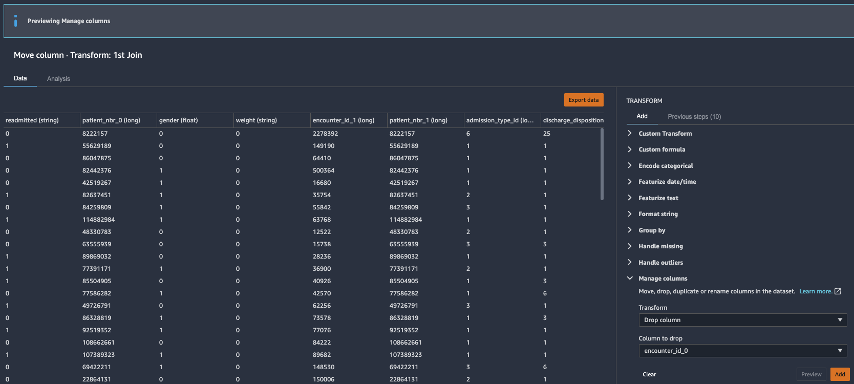
6. Repeat these steps for the other redundant columns: patient_nbr_0, encounter_id_1, and patient_nbr_1.

At this stage, we have done a few analyses and applied a few transformations on our raw input dataset. If we choose to preserve the transformed state of the input dataset, like checkpoint, you can do so by choosing Export data. This option allows you to persist the transformed dataset to an S3 bucket.

Quick Model analysis

Now that we have applied transformations to our initial dataset, let’s explore the Quick Model analysis feature. Quick model helps you quickly evaluate the training dataset and produce importance scores for each feature. A feature importance score indicates how useful a feature is at predicting a target label. The feature importance score is between 0–1; a higher number indicates that the feature is more important to the whole dataset. Because our use case relates to the classification problem type, the quick model also generates an F1 score for the current dataset.

1. Switch back to Analysis Tab and click Create new analysis to bring-up built-in analysis
2. For Analysis type, choose Quick Model.
3. Enter a name for your analysis.
4. For Label, choose readmitted.
   
5. Choose Preview and wait for the model to be trained and the results to appear.

The resulting quick model F1 score shows 0.618 (your generated score might be different) with the transformed dataset. Data Wrangler performs several steps to generate the F1 score, including preprocessing, training, evaluating, and finally calculating feature importance. For more details about these steps, see Quick Model.

With the quick model analysis feature, data scientists can iterate through applicable transformations until they have their desired transformed dataset that can potentially lead to better business accuracy and expectations.

6. Choose Save to add the quick model analysis to the data flow.

Export options

We’re now ready to export our data flow for further processing.

1. Navigate back to data flow designer by clicking Back to data flow on the top left
2. On the Export tab, choose Steps to reveal the Data Wrangler flow steps.
3. Choose the last step to mark it with a check.
   
4. Choose Export step to reveal the export options.

As of this writing, you have four export options:

• Save to S3 – Save the data to an S3 bucket using a SageMaker processing job
• Pipeline – Export a Jupyter notebook that creates a SageMaker pipeline with your data flow
• Python Code – Export your data flow to Python code
• Feature Store – Export a Jupyter notebook that creates a Feature Store feature group and adds features to an offline or online feature store
  

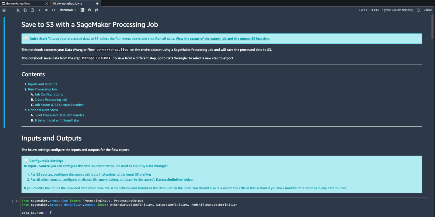
5. Choose Save to S3 to generate a fully implemented Jupyter notebook that creates a processing job using your data flow file.
   

Run processing and training jobs for model building

In this section, we show how to run processing and training jobs using the generated Jupyter notebook from Data Wrangler.

Submit a processing job

We’re now ready to submit a SageMaker processing job using our data flow file.

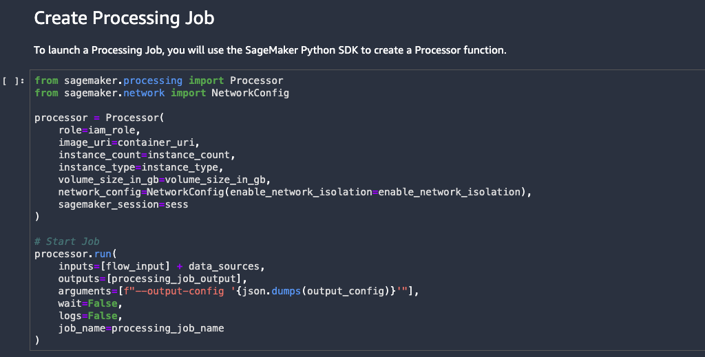
Run all the cells up to and including the Create Processing Job cell inside the exported notebook.

The cell Create Processing Job triggers a new SageMaker processing job by provisioning managed infrastructure and running the required Data Wrangler Docker container on that infrastructure.

You can check the status of the submitted processing job by running the next cell Job Status & S3 Output Location.

You can also check the status of the submitted processing job on the SageMaker console.

Train a model with SageMaker

Now that the data has been processed, let’s train a model using the data. The same notebook has sample steps to train a model using the SageMaker built-in XGBoost algorithm. Because our use case is a binary classification ML problem, we need to change the objective to binary:logistic inside the sample training steps.

Now we’re ready to run our training job using the SageMaker managed infrastructure. Run the cell Start the Training Job.

You can monitor the status of the submitted training job on the SageMaker console, on the Training jobs page.

Host a trained model for real-time inference

We now use another notebook available on GitHub under the project folder hosting/Model_deployment_Steps.ipynb. This is a simple notebook with two cells: the first cell has code for deploying your model to a persistent endpoint. You need to update model_url with your training job output S3 model artifact.

The second cell in the notebook runs inference on the sample test file under test_data/test_data_UCI_sample.csv. As you can see, we are able to generate predictions for our synthetic observations inside csv file. That concludes the ML workflow.

Clean up

After you have experimented with the steps in this post, perform the following cleanup steps to stop incurring charges:

1. On the SageMaker console, under Inference in the navigation pane, choose Endpoints.
2. Select your hosted endpoint.
3. On the Actions menu, choose Delete.
   
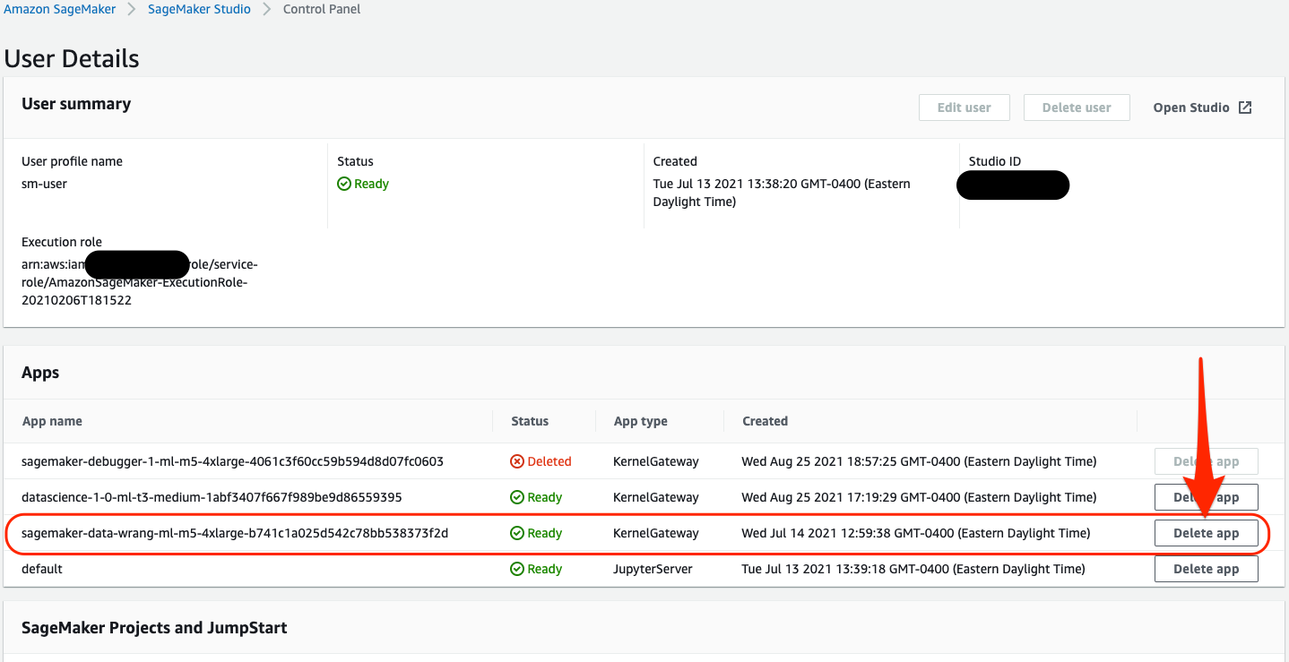
4. On the SageMaker Studio Control Panel, navigate to your SageMaker user profile.
5. Under Apps, locate your Data Wrangler app and choose Delete app.
   

Conclusion

In this post, we explored Data Wrangler capabilities using a public medical dataset related to patient readmission and demonstrated how to perform feature transformations using built-in transforms and quick analysis. We showed how, without much coding, to generate the required steps to trigger data processing and ML training. This no-code/low-code capability of Data Wrangler accelerates training data preparation and increases data scientist agility with faster iterative data preparation. In the end, we hosted our trained model and ran inferences against synthetic test data. We encourage you to check out our GitHub repository to get hands-on practice and find new ways to improve model accuracy! To learn more about SageMaker, visit the SageMaker Development Guide.

About the Authors

Shyam Namavaram is a Senior Solutions Architect at AWS. He has over 20 years of experience architecting and building distributed, hybrid, and cloud-native applications. He passionately works with customers accelerating their AI/ML adoption by providing technical guidance and helping them innovate and build secure cloud solutions on AWS. He specializes in AI/ML, containers, and analytics technologies. Outside of work, he loves playing sports and exploring nature with trekking.

Michael Hsieh is a Senior AI/ML Specialist Solutions Architect. He works with customers to advance their ML journey with a combination of Amazon ML offerings and his ML domain knowledge. As a Seattle transplant, he loves exploring the great nature the region has to offer, such as the hiking trails, scenery kayaking in the SLU, and the sunset at the Shilshole Bay.