Bring your own container to project model accuracy drift with Amazon SageMaker Model Monitor

AWS Feed
Bring your own container to project model accuracy drift with Amazon SageMaker Model Monitor

The world we live in is constantly changing, and so is the data that is collected to build models. One of the problems that is often seen in production environments is that the deployed model doesn’t behave the same way as it did during the training phase. This concept is generally called data drift or dataset shift, and can be caused by many factors, such as bias in sampling data that affects features or label data, the non-stationary nature of time series data, or changes in the data pipeline. Because machine learning (ML) models aren’t deterministic, it’s important to minimize the variance in the production environment by periodically monitoring the deployment environment for model drift and sending alerts and, if necessary, triggering retraining of the models with new data.

Amazon SageMaker is a fully managed service that enables developers and data scientists to quickly and easily build, train, and deploy ML models at any scale. After you train an ML model, you can deploy it on SageMaker endpoints that are fully managed and can serve inferences in real time with low latency. After you deploy your model, you can use Amazon SageMaker Model Monitor to continuously monitor the quality of your ML model in real time. You can also configure alerts to notify and trigger actions if any drift in model performance is observed. Early and proactive detection of these deviations enables you to take corrective actions, such as collecting new ground truth training data, retraining models, and auditing upstream systems, without having to manually monitor models or build additional tooling.

In this post, we present some techniques to detect covariate drift (one of the types of data drift) and demonstrate how to incorporate your own drift detection algorithms and visualizations with Model Monitor.

Types of data drift

Data drift can be classified into three categories depending on whether the distribution shift is happening on the input or on the output side, or whether the relationship between the input and the output has changed.

Covariate shift

In a covariate shift, the distribution of inputs changes over time, but the conditional distribution P(y|x) doesn’t change. This type of drift is called covariate shift because the problem arises due to a shift in the distribution of the covariates (features). For example, the training dataset for a face recognition algorithm may contain predominantly younger faces, while the real world may have a much larger proportion of older people.

Label shift

While covariate shift focuses on changes in the feature distribution, label shift focuses on changes in the distribution of the class variable. This type of shifting is essentially the reverse of covariate shift. An intuitive way to think about it might be to consider an unbalanced dataset; for example, if the spam to non-spam ratio of emails in our training set is 50%, but in reality, 10% of our emails are non-spam, then the target label distribution has shifted.

Concept shift

Concept shift is different from covariate and label shift in that it’s not related to the data distribution or the class distribution, but instead is related to the relationship between the two variables. For example, in stock analysis, the relationship between prior stock market data and the stock price is non-stationary. The relationship between the input data and the target variable changes over time, and the model needs to be refreshed often.

Now that we know the types of distribution shifts, let’s see how Model Monitor helps us in detecting data drifts. In the next section, we walk through setting up Model Monitor and incorporating our custom drift detection algorithms.

Model Monitor

Model Monitor offers four different types of monitoring capabilities to detect and mitigate model drift in real time:

• Data quality – Helps detect change in data schemas and statistical properties of independent variables and alerts when a drift is detected.
• Model quality – For monitoring model performance characteristics such as accuracy or precision in real time, Model Monitor allows you to ingest the ground truth labels collected from your applications. Model Monitor automatically merges the ground truth information with prediction data to compute the model performance metrics.
• Model bias –Model Monitor is integrated with Amazon SageMaker Clarify to improve visibility into potential bias. Although your initial data or model may not be biased, changes in the world may cause bias to develop over time in a model that has already been trained.
• Model explainability – Drift detection alerts you when a change occurs in the relative importance of feature attributions.

Deequ, which measures data quality, powers some of the Model Monitor pre-built monitors. You don’t require coding to utilize these pre-built monitoring capabilities. You also have the flexibility to monitor models by coding to provide custom analysis. All metrics emitted by Model Monitor can be collected and viewed in Amazon SageMaker Studio, so you can visually analyze your model performance without writing additional code.

In certain scenarios, the pre-built monitors may not be sufficient to generate sophisticated metrics to detect drifts, and may necessitate bringing your own metrics. In the next sections, we describe the setup to bring in your metrics by building a custom container.

Environment setup

For this post, we use a SageMaker notebook to set up Model Monitor and also visualize the drifts. We begin with setting up required roles and Amazon Simple Storage Service (Amazon S3) buckets to store our data:

region = boto3.Session().region_name sm_client = boto3.client('sagemaker') role = get_execution_role()
print(f"RoleArn: {role}") # You can use a different bucket, but make sure the role you chose for this notebook
# has the s3:PutObject permissions. This is the bucket into which the data is captured
bucket = session.Session(boto3.Session()).default_bucket()
print(f"Demo Bucket: {bucket}")
prefix = 'sagemaker/DEMO-ModelMonitor' s3_capture_upload_path = f's3://{bucket}/{prefix}/datacapture'
s3_report_path = f's3://{bucket}/{prefix}/reports'

Upload train dataset, test dataset, and model file to Amazon S3

Next, we upload our training and test datasets, and also the training model we use for inference. For this post, we use the Census Income Dataset from UCI Machine Learning Repository. The dataset consists of people’s income and several attributes that describe population demographics. The task is to predict if a person makes above or below $50,000. This dataset contains both categorical and integral attributes, and has several missing values. This makes it a good example to demonstrate model drift and detection.

We use XGBoost algorithm to train the model offline using SageMaker. We provide the model file for deployment. The training dataset is used for comparing with inference data to generate drift scores, while test dataset is used for computing how much the accuracy of the model has degraded due to drift. We provide more intuition on these algorithms in later steps.

The following code uploads our datasets and model to Amazon S3:

model_file = open("model/model.tar.gz", 'rb')
train_file = open("data/train.csv", 'rb')
test_file = open("data/test.csv", 'rb') s3_model_key = os.path.join(prefix, 'model.tar.gz')
s3_train_key = os.path.join(prefix, 'train.csv')
s3_test_key = os.path.join(prefix, 'test.csv') boto3.Session().resource('s3').Bucket(bucket).Object(s3_model_key).upload_fileobj(model_file)
boto3.Session().resource('s3').Bucket(bucket).Object(s3_train_key).upload_fileobj(train_file)
boto3.Session().resource('s3').Bucket(bucket).Object(s3_test_key).upload_fileobj(test_file)

Set up a Docker container

Model Monitor supports bringing your own custom model monitor containers. When you create a MonitoringSchedule, Model Monitor starts processing jobs for evaluating incoming inference data. While invoking the containers, Model Monitor sets up additional environment variables for you so that your container has enough context to process the data for that particular run of the scheduled monitoring. For the container code variables, see Container Contract Inputs. Of the available input environmental variables, we’re interested in dataset_source, output_path, and end_time:

"Environment": { "dataset_source": "/opt/ml/processing/endpointdata", "output_path": "/opt/ml/processing/resultdata", "end_time": "2019-12-01T16: 20: 00Z"
}

The dataset_source variable specifies the data capture location on the container, and end_time refers to the time of the last event capture. The custom drift algorithm is included in the src directory. For details on the algorithms, see the GitHub repo.

Now we build the Docker container and push it to Amazon ECR. See the following Dockerfile:

FROM python:3.8-slim-buster RUN pip3 install pandas==1.1.4 numpy==1.19.4 scikit-learn==0.23.2 pyarrow==2.0.0 scipy==1.5.4 boto3==1.17.12 WORKDIR /home
COPY src/* /home/ ENTRYPOINT ["python3", "drift_detector.py"]

We build and push it to Amazon ECR with the following code:

from docker_utils import build_and_push_docker_image repository_short_name = 'custom-model-monitor' image_name = build_and_push_docker_image(repository_short_name)

Set up an endpoint and enable data capture

As we mentioned before, our model was trained using XGBoost, so we use XGBoostModel from the SageMaker SDK to deploy the model. Because we have a custom input parser, which includes imputation and one-hot encoding, we provide the inference entry point along with source directory, which includes the Scikit ColumnTransfomer model. The following code is the customer inference function:

script_path = pathlib.Path(__file__).parent.absolute()
with open(f'{script_path}/preprocess.pkl', 'rb') as f: preprocess = pickle.load(f) def input_fn(request_body, content_type): """ The SageMaker XGBoost model server receives the request data body and the content type, and invokes the `input_fn`. Return a DMatrix (an object that can be passed to predict_fn). """ if content_type == 'text/csv': df = pd.read_csv(StringIO(request_body), header=None) X = preprocess.transform(df) X_csv = StringIO() pd.DataFrame(X).to_csv(X_csv, header=False, index=False) req_transformed = X_csv.getvalue().replace('n', '') return xgb_encoders.csv_to_dmatrix(req_transformed) else: raise ValueError( f'Content type {request_content_type} is not supported.' )

We also include the configuration for data capture, specifying the S3 destination, and sampling percentage with the endpoint deployment (see the following code). Ideally, we want to capture 100% of the incoming data for drift detection, but for a high traffic endpoint, we suggest reducing the sampling percentage so that the endpoint availability isn’t affected. Besides, Model Monitor might automatically reduce the sampling percentage if it senses the endpoint availability is affected.

from sagemaker.xgboost.model import XGBoostModel
from sagemaker.serializers import CSVSerializer
from sagemaker.model_monitor import DataCaptureConfig model_url = f's3://{bucket}/{s3_model_key}' xgb_inference_model = XGBoostModel( model_data=model_url, role=role, entry_point='inference.py', source_dir='script', framework_version='1.2-1',
) data_capture_config = DataCaptureConfig( enable_capture=True, sampling_percentage=100, destination_s3_uri=s3_capture_upload_path) predictor = xgb_inference_model.deploy( initial_instance_count=1, instance_type='ml.c5.xlarge', serializer=CSVSerializer(), data_capture_config=data_capture_config)

After we deploy the model, we can set up a monitor schedule.

Create a monitor schedule

Typically, we create a processing job to generate baseline metrics of our training set. Then we create a monitor schedule to start periodic jobs to analyze incoming inference requests and generate metrics similar to baseline metrics. The inference metrics are compared with baseline metrics and a detailed report on constraints violation and drift in data quality is generated. Using SageMaker SDK simplifies the creation of baseline metrics and scheduling model monitor.

For the algorithms we use in this post (such as Wasserstein distance and Kolmogorov–Smirnov test), the container that we build needs access to both the training dataset and the inference data for computing metrics. This non-typical setup requires some low-level setup of the monitor schedule. The following code is the Boto3 request to set up the monitor schedule. The key fields are related to the container image URL and arguments to the container. We cover building containers in the next section. For now, note that we pass the S3 URL for training the dataset:

s3_train_path = f's3://{bucket}/{s3_train_key}'
s3_test_path = f's3://{bucket}/{s3_test_key}'
s3_result_path = f's3://{bucket}/{prefix}/result/{predictor.endpoint_name}' sm_client.create_monitoring_schedule( MonitoringScheduleName=predictor.endpoint_name, MonitoringScheduleConfig={ 'ScheduleConfig': { 'ScheduleExpression': 'cron(0 * ? * * *)' }, 'MonitoringJobDefinition': { 'MonitoringInputs': [ { 'EndpointInput': { 'EndpointName': predictor.endpoint_name, 'LocalPath': '/opt/ml/processing/endpointdata' } }, ], 'MonitoringOutputConfig': { 'MonitoringOutputs': [ { 'S3Output': { 'S3Uri': s3_result_path, 'LocalPath': '/opt/ml/processing/resultdata', 'S3UploadMode': 'EndOfJob' } }, ] }, 'MonitoringResources': { 'ClusterConfig': { 'InstanceCount': 1, 'InstanceType': 'ml.c5.xlarge', 'VolumeSizeInGB': 10 } }, 'MonitoringAppSpecification': { 'ImageUri': image_name, 'ContainerArguments': [ '--train_s3_uri', s3_train_path, '--test_s3_uri', s3_test_path, '--target_label', 'income' ] }, 'StoppingCondition': { 'MaxRuntimeInSeconds': 600 }, 'Environment': { 'string': 'string' }, 'RoleArn': role } }
)

Generate requests for the endpoint

After we deploy the model, we send traffic at a constant rate to the endpoints. The following code launches a thread to generate the requests for about 10 hours. Make sure to stop the kernel if you want to stop the traffic. We let the traffic generator run for a few hours to collect enough samples to visualize drift. The plots automatically refresh whenever there is new data.

def invoke_endpoint(ep_name, file_name, runtime_client): pre_time = time() with open(file_name) as f: count = len(f.read().split('n')) - 2 # Remove EOF and header # Calculate time needed to sleep between inference calls if we need to have a constant rate of calls for 10 hours ten_hours_in_sec = 10*60*60 sleep_time = ten_hours_in_sec/count with open(file_name, 'r') as f: next(f) # Skip header for ind, row in enumerate(f): start_time = time() payload = row.rstrip('n') response = runtime_client(data=payload) # Print every 15 minutes (900 seconds) if (ind+1) % int(count/ten_hours_in_sec*900) == 0: print(f'Finished sending {ind+1} records.') # Sleep to ensure constant rate. Time spent for inference is subtracted sleep(max(sleep_time - (time() - start_time), 0)) print("Done!") print(f"Sending test traffic to the endpoint {predictor.endpoint_name}.nPlease wait...") thread = Thread(target = invoke_endpoint, args=(predictor.endpoint, 'data/infer.csv', predictor.predict))
thread.start()

Visualize the data drift

We use the entire dataset for training and synthetically generate a new dataset for inference by modifying statistical properties of some of the attributes from the original dataset as described in our GitHub repo.

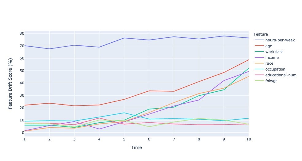
Normalized drift score per feature

A normalized drift score (in %) for each feature is computed by calculating the ratio of overlap of the distribution of incoming inference data with the original data to the original data. For categorical data, this is computed by summing the absolute of the difference in probability scores (training and inference) across each label. For numerical data, the training data is split into 10 bins (deciles), and the absolute of the difference in probability scores over bin is summed to calculate the drift score.

The following plot shows the drift scores over the time intervals. A few features have low to no drifts, while some features have drifts that are increasing over time, and finally hours-per-week has a large drift right from the start.

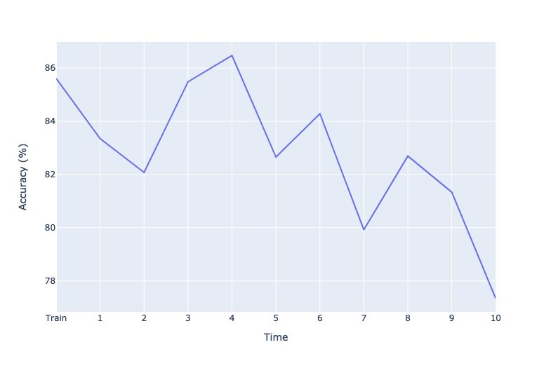
Projected drift in model accuracy

This metric provides a proxy of the accuracy of a model due to drift in inference data from the test data. The idea behind this approach is to determine how much percentage of the inference data is similar to the portion of the test data, where the model predicts well. For this metric, we use Isolation Forests to train one-class classifier, and generate scores for the portion of the test data that model predicted well, and for the inference data. The relative difference in the mean of these scores is the projected drift in accuracy.

The following plot shows the corresponding degradation in model accuracy due to drift in the incoming data. This demonstrates that covariate shift can reduce accuracy of a model. A few spikes in the metric can be attributed to the statistical nature of how the data is generated. This is only a proxy for model accuracy, and not the actual accuracy, which can only be known from the ground truth of the labels.

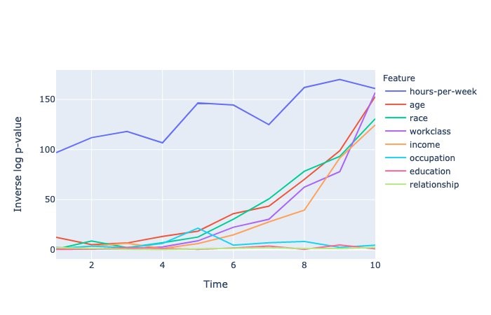
P-values of null test hypothesis

A null test hypothesis tests whether two samples (for this post, the training and inference datasets) are derived from the same general population. The p-value gives the probability of obtaining test results at least as extreme as the observations under the assumption that the null hypothesis is correct. A p-value threshold of 5% is used to decide whether the observed sample has drifted from the training data or not.

The following plot shows p-values of different attributes that have crossed the threshold at least once. The y-axis shows the inverse log of p-values to distinguish very small p-values. P-values for numerical attributes are obtained from Kolmogorov–Smirnov test, and for categorical attributes from Chi-square test.

Conclusion

Amazon SageMaker Model Monitor is a powerful tool to detect data drift. In this post, we showed how to easily integrate your custom data drift detection algorithms into Model Monitor, while benefiting from the heavy lifting that Model Monitor provides in terms of data capture and scheduling the monitor runs. The notebook provides a detailed step-by-step instruction on how to build a custom container and attach it to Model Monitor schedules. Give Model Monitor a try and leave your feedback in the comments.

About the Author

Vinay Hanumaiah is a Senior Deep Learning Architect at Amazon ML Solutions Lab, where he helps customers build AI and ML solutions to accelerate their business challenges. Prior to this, he contributed to the launch of AWS DeepLens and Amazon Personalize. In his spare time, he enjoys time with his family and is an avid rock climber.