AWS Feed
Deepset achieves a 3.9x speedup and 12.8x cost reduction for training NLP models by working with AWS and NVIDIA

This is a guest post from deepset (creators of the open source frameworks FARM and Haystack), and was contributed to by authors from NVIDIA and AWS.
At deepset, we’re building the next-level search engine for business documents. Our core product, Haystack, is an open-source framework that enables developers to utilize the latest NLP models for semantic search and question answering at scale. Our software as a service (SaaS) platform, Haystack Hub, is used by developers from various industries, including finance, legal, and automotive, to find answers in all kinds of text documents. You can use these answers to improve the search experience, cover the long-tail of chat bot queries, extract structured data from documents, or automate invoicing processes.
Pretrained language models like BERT, RoBERTa, and ELECTRA form the core for this latest type of semantic search and many other NLP applications. Although plenty of English models are available, the availability for other languages and more industry-specific terms (such as finance or automotive) is usually very limited and often complicates applications in the industry. Therefore, we regularly train language models for languages not covered by existing models (such as German BERT and German ELECTRA), models for special domains (such as finance and aerospace), or even models for client-specific jargon.
Challenge
Pretraining language models from scratch typically involves two major challenges: cost and development effort.
Training a language model is an extremely compute-intensive task and requires multiple GPUs running for multiple days. To give you a rough idea, training the original RoBERTa model took about 1 day on 1024 NVIDIA V100 GPUs.
Computation costs aren’t the only thing that can stress your budget. A considerable amount of manual development is required to create the training data and vocabulary, configure hyperparameters, start and monitor training jobs, and run periodical evaluation of different model checkpoints. In our first training runs, we also found several bugs only after multiple hours of training, resulting in a slow development cycle. In summary, language model training can be a painful job for a developer and easily consumes multiple days of work.
Solution
In a collaborative effort, AWS, NVIDIA, and deepset were able to complete training 3.9 times faster while lowering cost by 12.8 times and reducing developer effort from days to hours. We optimized the GPU utilization during training via PyTorch’s DistributedDataParallel (DDP) and enabled larger batch sizes by switching to Automatic Mixed Precision (AMP). Furthermore, we introduced a StreamingDataSilo that allows us to load the training data lazily from disk and to do the preprocessing on the fly, leading to a lower memory footprint and no initial preprocessing time. Last but not least, we integrated the training with Amazon SageMaker to reduce manual development effort and benefit from around a 70% cost reduction by using Amazon Elastic Compute Cloud (Amazon EC2) Spot Instances.
In this post, we explore each of these technologies and their impact on improving BERT training performance.
DistributedDataParallel
DistributedDataParallel (DDP) implements distributed data parallelism in PyTorch. This is a key module that’s essential for running training jobs at scale, on multiple machines or on multiple GPUs in a single machine. DDP parallelizes a given network module by splitting the input across specified devices (GPUs). The input is split in the batch dimension. The network module is replicated on each device, and each such replica handles a slice of the input. The gradients from each device are averaged during a backward pass. DDP is used in conjunction with the torch.distributed framework, which handles all communication and synchronization in distributed training jobs with PyTorch.
Before DDP was introduced, torch.nn.DataParallel (DP) was the standard module for doing single-machine multi-GPU training in PyTorch. The system in DP works as follows:
- The entire batch of input is loaded on the main thread.
- The batch is split and scattered across all the GPUs in the network.
- Each GPU runs the forward pass on its batch, split on a separate thread.
- The network outputs are gathered on the master GPU, the loss value is computed, and this loss value is then scattered across the other GPUs.
- Each GPU uses the loss value to run a backward pass and compute the gradients.
- The gradients are reduced on the master GPU and the model parameters on the master GPU are updated. This completes one iteration of training.
- To ensure all GPUs have the latest model parameters, they are broadcasted to the other GPUs at the start of the next iteration.
This design of DP has several inefficiencies:
- Uneven GPU utilization – Only the primary GPU handles loss calculation, gradient reduction, and parameter updates, which leads to higher GPU memory consumption compared to the rest of the GPUs
- Unnecessary broadcast at the beginning of each iteration – Because the model parameters are only updated in the master GPU, they need to be broadcast to the other GPUs before every iteration
- Unnecessary gathering step – There is an unnecessary gathering step of model outputs on the GPU
- Redundant data copies – Data is first copied to the master GPU, which is then split and copied over to the other GPUs
- Multithreading overhead – Performance overhead caused by the Global Interpreter Lock (GIL) of the Python interpreter
DDP eliminates all such inefficiencies of DP. DDP uses a multiprocessing architecture, unlike the multithreaded one in DP. This means each GPU has its own dedicated process which runs independently and there is no master GPU anymore. Each process starts by loading its own split of data from the disk. Then the forward pass and loss computation is run independently on each GPU. This eliminates the need for gathering network outputs. During the backward pass, the gradients are AllReduced across the GPUs. Averaging the gradients with AllReduce ensures that the gradients in each GPU are identical. As a result, the model updates in each GPU are identical as well, which eliminates the need for parameter broadcast at the start of the next iteration.
Results with DDP
With DP, the GPU memory utilization was skewed towards the master GPU, which consumed 15 GB, whereas all other GPUs consumed 6 GB. With DDP, the memory consumption was split equally across 4 GPUs, or about 9 GB on each. This also allowed us to increase the per GPU batch size, which further contributed to the speedup in throughput. We reduced the number of gradient accumulation steps to keep the effective batch size constant, to ensure that there was no impact in convergence.
The following table shows the results on a P3.8xlarge instance with 4 NVIDIA V100 GPUs. With DDP, the training time reduced from 616 hours to 347 hours.
| Run | Batch Size | Accumulation Steps | Effective Batch Size | Throughput (Effective Batches per Hour) | Total Estimated Training Time (Hours) |
| BERT Training with DP | 105 | 9 | 945 | 811 | 616 |
| BERT Training with DDP | 240 | 4 | 960 | 1415 | 347 |
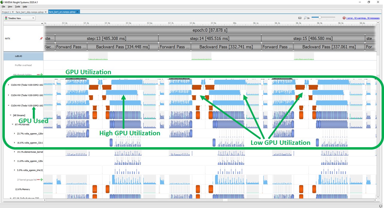
The following screenshots show the GPU performance profiles captured by the NVIDIA Nsight Systems. The first screenshot shows the profile while running with DP. Light blue bars in the box marked as “GPU Utilization” show if GPUs are busy. Gaps between the blue areas show that the GPU utilization is zero. The red blocks in between are CPU to GPU memory copy operations. An additional blue block is between the memory copies, which is the aggregation operation that is computed on a single GPU.

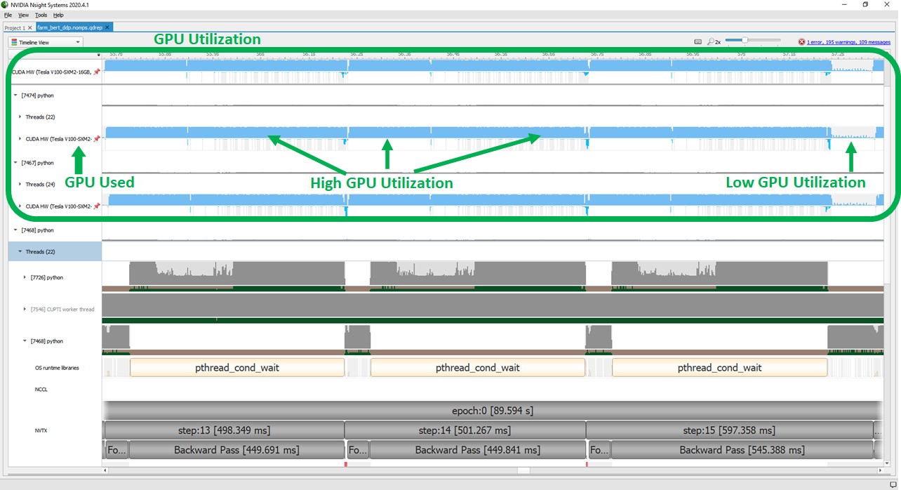
The following screenshot shows high GPU utilization with DDP, which effectively deprecates all those inefficiencies.

Training with Automatic Mixed Precision
Automatic Mixed Precision (AMP) speeds up deep learning training with minimal impact to final accuracy. Traditionally, 32-bit precision floating point (FP32) variables are commonly used in deep learning training. You can improve speed of training with 16-bit precision floating point (FP16) variables because it requires lower storage and less memory bandwidth. However, training with lower precision could decrease the accuracy of the results. Mixed precision training is a balanced approach to achieve the computational speed up of lower precision training while maintaining accuracy close to FP32 precision training. Training with mixed precision provides additional speedup by using NVIDIA Tensor Cores, which are specialized hardware available on NVIDIA GPUs for accelerated computation.
To maintain accuracy, training with mixed precision involves the following steps:
- Port the model to use the FP16 datatype where appropriate.
- Handle specific functions or operations that must be done in FP32 to maintain accuracy.
- Add loss scaling to preserve small gradient values.
The AMP feature handles all these steps for deep learning training. As of this writing, all popular deep learning frameworks like PyTorch, TensorFlow, and Apache MXNet support AMP.
AMP in PyTorch was supported via the NVIDIA APEX library. AMP support has recently been moved to PyTorch core with the 1.6 release.
AMP in APEX library provides four levels of optimization for different application usage. Optimization levels O1 and O2 are both mixed precision modes with slight differences, where O1 is the recommended way for typical use cases and 02 is more aggressively converting most layers into FP16 mode. O0 and O4 opt levels are actually the FP32 mode and FP16 mode designed for reference only.
The following table shows the impact of applying AMP along with DDP. Without AMP, batch size up to 240 could be run on the GPU. With AMP, the larger batch size of 320 could be supported, reducing the total training time from 347 hours to 223 hours
| Run | Batch Size | Accumulation Steps | Effective Batch Size | Throughput (Effective Batches per Hour) | Total Estimated Training Time (Hours) |
| BERT Training with DDP | 240 | 4 | 960 | 1415 | 347 |
| BERT Training with DDP & AMP 01 | 304 | 3 | 912 | 2025 | 243 |
| BERT Training with DDP & AMP 02 | 320 | 3 | 960 | 2210 | 223 |
As mentioned earlier, AMP O2 converts more layers into FP16 mode, so we can run DDP and AMP O2 with a larger batch size and get a better throughput compared to DDP and AMP O1. When selecting between these two opt levels, you should do a validation of the prediction results to make sure AMP O2 meets your accuracy requirements.
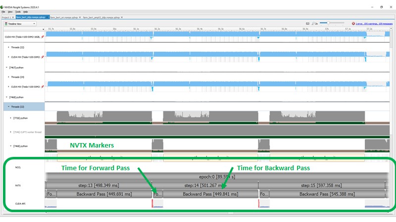
The following screenshot shows the GPU performance profile after applying DDP but running the deep learning training with FP32 variables. In this profile, we have added custom markers called NVTX markers, which show the time taken for each epoch, each step, and the time for the forward and backward pass.

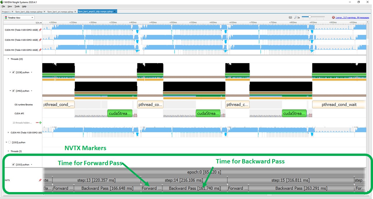
The following screenshot shows the profile after enabling AMP with opt level O2. The time to run a forward and backward pass reduced significantly even though we increased the batch size for training when using AMP.

Earlier, we mentioned that AMP utilizes Tensor Cores available on NVIDIA GPU hardware for significant speedup for deep learning training. GPU performance profiles show when operations are utilizing Tensor Cores. The following screenshot shows a sample GPU kernel that is run in FP32 mode. The GPU operation is marked here as the volta_sgemm kernel.

The following screenshot shows similar operations run in FP16 mode, which utilizes Tensor Cores. Kernels running with Tensor Cores are marked as volta_fp16_s884gemm.

Data pipeline
The datasets used for training language models typically contain 10–200 GB of raw text data. Loading the whole dataset in RAM can be challenging. Furthermore, the typical pipeline of first running the preprocessing for all data and then pulling batches during training isn’t optimal because the up-front preprocessing can take multiple hours in which we don’t utilize the GPUs on the server.
Therefore, we introduced a StreamingDataSilo, which loads data lazily from disk just in time when it’s needed in the training loop. The whole preprocessing happens on the fly. Our implementation builds upon PyTorch’s IterableDataset and DistributedSampler, but requires some custom parts to ensure enough preprocessed batches are always in the queue for our trainer, so that the GPU never has to wait for the next batch to be ready. For implementation steps, see the GitHub repo. Together with an increased number of workers to fill the queue, we ended up with another 28% throughput improvement, as shown in the following table.
| Run | Batch Size | Accumulation Steps | Effective Batch Size | Throughput (Effective Batches per Hour) | Total Estimated Training Time (Hours) |
| DDP with 8 workers | 320 | 3 | 960 | 2210 | 223 |
| DDP with 16 workers | 320 | 3 | 960 | 3077 | 160 |
A second tricky case that we had to handle was related to the unknown number of batches in our dataset and the distributed training via DDP. If the batches in your dataset can’t be evenly distributed across the number of workers, some workers don’t get any batches in the last step of the epoch while others do. This asynchronicity can crash your whole training run or result in a deadlock (for a related PyTorch issue, see [RFC] Join-based API to support uneven inputs in DDP). We handled this by adding a small synchronization step where all workers communicate if they still have data left. For implementation details, see the GitHub repo.
Spot Instances
Besides reducing the total training time, using EC2 Spot Instances is another compelling approach to reduce training costs. This is pretty straightforward to configure in SageMaker; just set the parameter EnableManagedSpotTraining to True when launching your training job. SageMaker launches your training job and saves checkpoints periodically. When your Spot Instance ends, SageMaker takes care of spinning up a new instance and loading the latest checkpoint to continue training from there.
In your code, you need to make sure to save regular checkpoints containing the states of all the objects that are relevant for your training session. This includes not only your model weights, but also the states of your optimizer, the data loader, and all random number generators to replicate the results from your continuous runs without Spot Instances. For implementation details, see the GitHub repo.
In our test runs, we achieved around 70% cost savings in comparison to regular On-Demand Instances.
Conclusion
Language models have become the backbone of modern NLP. Although using existing public models works well in many cases, many domains with special languages can benefit from training a new model from scratch. Having a fast, simple, and cheap training pipeline is essential for these big training jobs. In addition, the increased efficiency of training jobs reduces our energy usage and lowers our carbon footprint. By tackling different areas of FARM’s training pipeline, we were able to significantly optimize the resource utilization. In the end, we were able to achieve a speedup in training time of 3.9 times faster, a 12.8 times reduction in training cost, and reduced the developer effort required from days to hours.
If you’re interested in training your own BERT model, you can look at the open-source code in FARM or try our free SageMaker algorithm on the AWS Marketplace.
About the Authors
Abhinav Sharma is a Software Engineer at AWS Deep Learning. He works on bringing state-of-the-art deep learning research to customers, building products that help customers use deep learning engines. Outside of work, he enjoys playing tennis, noodling on his guitar and watching thriller movies.
Malte Pietsch is Co-Founder & CTO at deepset, where he builds the next-level enterprise search engine fueled by open source and NLP. He holds a M.Sc. with honors from TU Munich and conducted research at Carnegie Mellon University. He is an open-source lover, likes reading papers before breakfast, and is obsessed with automating the boring parts of our work.
Khaled ElGalaind is the engineering manager for AWS Deep Engine Benchmarking, focusing on performance improvements for AWS machine learning customers. Khaled is passionate about democratizing deep learning. Outside of work, he enjoys volunteering with the Boy Scouts, BBQ, and hiking in Yosemite.
Jiahong Liu is a Solution Architect on the NVIDIA Cloud Service Provider team, where he helps customers adopt ML and AI solutions with better utilization of NVIDIA’s GPU to solve their business challenges.
Anish Mohan is a Machine Learning Architect at NVIDIA and the technical lead for ML and DL engagements with key NVIDIA customers in the greater Seattle region. Before NVIDIA, he was at Microsoft’s AI Division, working to develop and deploy AI and ML algorithms and solutions.