Run distributed hyperparameter and neural architecture tuning jobs with Syne Tune

AWS Feed
Run distributed hyperparameter and neural architecture tuning jobs with Syne Tune

Today we announce the general availability of Syne Tune, an open-source Python library for large-scale distributed hyperparameter and neural architecture optimization. It provides implementations of several state-of-the-art global optimizers, such as Bayesian optimization, Hyperband, and population-based training. Additionally, it supports constrained and multi-objective optimization, and allows you to bring your own global optimization algorithm.

With Syne Tune, you can run hyperparameter and neural architecture tuning jobs locally on your machine or remotely on Amazon SageMaker by changing just one line of code. The former is a well-suited backend for smaller workloads and fast experimentation on local CPUs or GPUs. The latter is well-suited for larger workloads, which come with a substantial amount of implementation overhead. Syne Tune makes it easy to use SageMaker as a backend to reduce wall clock time by evaluating a large number of configurations on parallel Amazon Elastic Compute Cloud (Amazon EC2) instances, while taking advantage of SageMaker’s rich set of functionalities (including pre-built Docker deep learning framework images, EC2 Spot Instances, experiment tracking, and virtual private networks).

By open-sourcing Syne Tune, we hope to create a community that brings together academic and industrial researchers in machine learning (ML). Our goal is to create synergies between these two groups by enabling academics to easily validate small-scale experiments at larger scale and industrials to use a broader set of state-of-the-art optimizers.

In this post, we discuss hyperparameter and architecture optimization in ML, and show you how to launch tuning experiments on your local machine and also on SageMaker for large-scale experiments.

Hyperparameter and architecture optimization in machine learning

Every ML algorithm comes with a set of hyperparameters that control the training algorithm or the architecture of the underlying statistical model. Typical examples of such hyperparameters for deep neural networks are the learning rate or the number of units per layer. Setting these hyperparameters correctly is crucial to obtain top-notch predictive performances.

To overcome the daunting process of trial and error, hyperparameter and architecture optimization aims to automatically find the specific configuration that maximizes the validation performance of our ML algorithm. Arguably, the easiest method to solve this global optimization problem is random search, where configurations are sampled from a predefined probability distribution. A more sample-efficient technique is Bayesian optimization, which maintains a probabilistic model of the objective function (here, the validation performance) to guide the search toward the global optimum in a sequential manner.

Unfortunately, with ever-increasing dataset sizes and ever-deeper models, training deep neural networks can be prohibitively slow to tune. Recent advances in hyperparameter optimization, such as Hyperband or MoBster, early stop the evaluation of configurations that are unlikely to achieve a good performance and reallocate the resources that would have been consumed to the evaluation of other candidate configurations. You can obtain further gains by using distributed resources to parallelize the tuning process. Because the time to train a deep neural network can vary widely across hyperparameter and architecture configurations, optimal resource allocation requires our optimizer to asynchronously decide which configuration to run next by taking the pending evaluation of other configurations into account. Next, we see how this works in practice and how we can run this either on a local machine or on SageMaker.

Tune hyperparameters with Syne Tune

We now detail how to tune hyperparameters with Syne Tune. First, you need a script that takes hyperparameters as arguments and reports results as soon as they are observed. Let’s look at a simplified example of a script that exposes the learning rate, dropout rate, and momentum as hyperparameters, and reports the validation accuracy after each training epoch:

from argparse import ArgumentParser
from syne_tune.report import Reporter if __name__ == '__main__': parser = ArgumentParser() parser.add_argument('--lr', type=float) parser.add_argument('--dropout_rate', type=float) parser.add_argument('--momentum', type=float) args, _ = parser.parse_known_args() report = Reporter() for epoch in range(1, args.epochs + 1): # ... train model and get validation accuracy val_acc = compute_accuracy() # Feed the score back to Syne Tune. report(epoch=epoch, val_acc=val_acc)

The important part is the call to report. It enables you to transmit results to a scheduler that decides whether to continue the evaluation of a configuration, or trial, and later potentially uses this data to select new configurations. In our case, we use a common use case that trains a computer vision model adapted from SageMaker examples on GitHub.

We define the search space for the hyperparameters (dropout, learning rate, momentum) that we want to optimize by specifying the ranges:

from syne_tune.search_space import loguniform, uniform max_epochs = 27
config_space = { "epochs": max_epochs, "lr": loguniform(1e-5, 1e-1), "momentum": uniform(0.8, 1.0), "dropout_rate": loguniform(1e-5, 1.0),
}

We also specify the scheduler we want to use, Hyperband in our case:

from syne_tune.optimizer.schedulers.hyperband import HyperbandScheduler scheduler = HyperbandScheduler( config_space, max_t=max_epochs, resource_attr='epoch', searcher='random', metric="val_acc", mode="max",
)

Hyperband is a method that randomly samples configurations and early stops evaluation trials if they’re not performing well enough after a few epochs. We use this particular scheduler for our example, but many others are available; for example, switching searcher=bayesopt enables us to use MoBster, which uses a surrogate model to sample new configurations to evaluate.

We’re now ready to define and launch a hyperparameter tuning job. First, we define the number of workers that evaluate trials concurrently and how long the optimization should run in seconds. Importantly, we use the local backend to evaluate our training script “train_cifar100.py” (see the full code). This means that the tuning happens on the local machine with one Python subprocess per worker. See the following code:

from syne_tune.backend.local_backend import LocalBackend
from syne_tune.tuner import Tuner
from syne_tune.stopping_criterion import StoppingCriterion tuner = Tuner( backend=LocalBackend(entry_point="train_cifar100.py"), scheduler=scheduler, stop_criterion=StoppingCriterion(max_wallclock_time=7200), n_workers=4,
) tuner.run()

As soon as the tuning starts, Syne Tune outputs the following line:

INFO:syne_tune.tuner:results of trials will be saved on /home/ec2-user/syne-tune/train-cifar100-2021-11-05-13-29-01-468

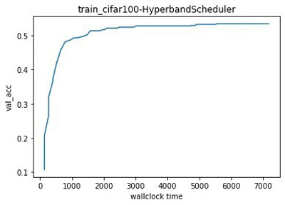
The log of the trials is stored in the aforementioned folder for further analysis. At any time during the tuning job, we can easily get the results obtained so far by calling load_experiment(“train-cifar100-2021-11-05-15-22-27-531”) and plotting the best result obtained since the start of the tuning job:

from syne_tune.experiments import load_experiment
tuning_experiment = load_experiment("train-cifar100-2021-11-05-15-22-27-531")
tuning_experiment.plot()

The following graph shows our results.

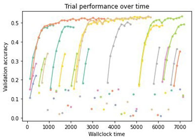
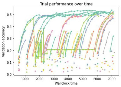
More fine-grained information is available if desired; the results obtained during tuning are stored as well as the scheduler and tuner state—namely, the state of the optimization process. For instance, we can plot the metric obtained for each trial over time (recall that we run four trials asynchronously). In the following figure, each trace represents the evaluation of a configuration as a function of the wall clock time; a dot is a trial stopped after one epoch.

We clearly see the effect of early stopping—only the most promising configurations are evaluated fully and poor performing configurations are stopped early, often after just evaluating a single epoch.

We can also easily switch to another scheduler, for example, random search or MoBster:

from syne_tune.optimizer.schedulers.fifo import FIFOScheduler scheduler = FIFOScheduler( config_space, searcher='random', metric="val_acc", mode="max",
)
scheduler = HyperbandScheduler( config_space, max_t=max_epochs, resource_attr='epoch', searcher='bayesopt', metric="val_acc", mode="max",
)

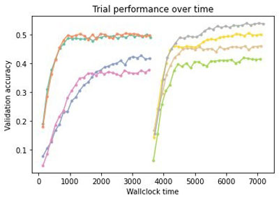
If we then run the same code with the new schedulers, we can compare all three methods. We see in the following figure that Hyperband only continues well-performing trials, and early stops poorly performing configurations.

Therefore, Hyperband evaluates many more configurations than random search (see the following figure), which uses resources to evaluate every configuration until the end. This can lead to drastic speedups of the tuning process in practice.

MoBster further improves over Hyperband by using a probabilistic surrogate model of the objective function.

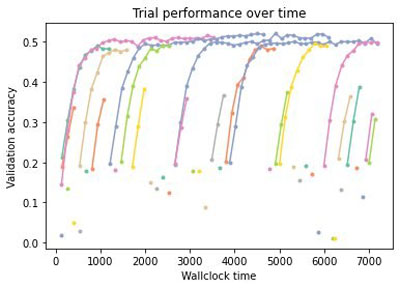
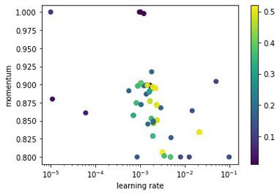
The following figure show all configurations that Hyperband samples during the tuning job.

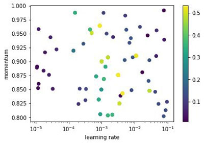
In comparison, MoBster samples more promising configurations around the well-performing range (brighter color being better) of the search space instead of sampling them uniformly at random like Hyperband.

Run large-scale tuning jobs with Syne Tune and SageMaker

The previous example showed how to tune hyperparameters on a local machine. Sometimes, we need more powerful machines or a large number or workers, which motivates the use of a cloud infrastructure. Syne Tune provides a very simple way to run tuning jobs on SageMaker. Let’s look at how this can be achieved with Syne Tune.

We first upload the cifar100 dataset to Amazon Simple Storage Service (Amazon S3) so that it’s available on EC2 instances:

import sagemaker sagemaker_session = sagemaker.Session()
bucket = sagemaker_session.default_bucket()
prefix = "sagemaker/DEMO-pytorch-cnn-cifar100"
role = sagemaker.get_execution_role()
inputs = sagemaker_session.upload_data(path="data", bucket=bucket, key_prefix="data/cifar100")

Next, we specify that we want trials to be run on the SageMaker backend. We use the SageMaker framework (PyTorch) in this particular example because we have a PyTorch training script, but you can use any SageMaker framework (such as XGBoost, TensorFlow, Scikit-learn, or Hugging Face).

A SageMaker framework is a Python wrapper that allows you to run ML code easily by providing a pre-made Docker image that works seamlessly on CPU and GPU for many framework versions. In this particular example, all we need to do is to instantiate the wrapper PyTorch with our training script:

from sagemaker.pytorch import PyTorch
from syne_tune.backend.sagemaker_backend.sagemaker_utils import get_execution_role
from syne_tune.backend.sagemaker_backend.sagemaker_backend import SagemakerBackend backend = SagemakerBackend( sm_estimator=PyTorch( entry_point="./train_cifar100.py", instance_type="ml.g4dn.xlarge", instance_count=1, role=get_execution_role(), framework_version='1.7.1', py_version='py3', ), inputs=inputs,
)

We can now run our tuning job again, but this time we use 20 workers, each having their own GPU:

tuner = Tuner( backend=backend, scheduler=scheduler, stop_criterion=StoppingCriterion(max_wallclock_time=7200, max_cost=20.0), n_workers=20, tuner_name="cifar100-on-sagemaker"
) tuner.run()

After each instance initiates a training job, you see the status update as in the local case. An important difference to the local backend is that the total estimated dollar cost is displayed as well the cost of workers.

trial_id status iter dropout_rate epochs lr momentum epoch val_acc worker-time worker-cost 0 InProgress 1 0.003162 30 0.001000 0.900000 1.0 0.4518 50.0 0.010222 1 InProgress 1 0.037723 30 0.000062 0.843500 1.0 0.1202 50.0 0.010222 2 InProgress 1 0.000015 30 0.000865 0.821807 1.0 0.4121 50.0 0.010222 3 InProgress 1 0.298864 30 0.006991 0.942469 1.0 0.2283 49.0 0.010018 4 InProgress 0 0.000017 30 0.028001 0.911238 - - - 5 InProgress 0 0.000144 30 0.000080 0.870546 - - - -
6 trials running, 0 finished (0 until the end), 387.53s wallclock-time, 0.04068444444444444$ estimated cost

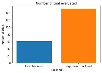
Because we specified max_wallclock_time=7200 and max_cost=20.0, the tuning job stops when the wall clock time or the estimated cost goes above the specified bound. In addition to providing an estimate of the cost, it can be optimized with our multi-objective optimizers (see the GitHub repo for an example). As shown in the following figures, the SageMaker backend allows you to evaluate many more configurations of hyperparameters and architectures in the same wall clock time than the local one and, as a result, increases the likelihood of finding a better configuration.

Conclusion

In this post, we saw how to use Syne Tune to launch tuning experiments on your local machine and also on SageMaker for large-scale experiments. To learn more about the library, check out our GitHub repo for documentation and examples that show, for instance, how to run model-based Hyperband, tune multiple objectives, or run with your own scheduler. We look forward to your contributions and seeing how this solution can address everyday tuning of ML pipelines and models.

About the Author

David Salinas is a Sr Applied Scientist at AWS.

 Aaron Klein is an Applied Scientist at AWS.

Matthias Seeger is a Principal Applied Scientist at AWS.

Cedric Archambeau is a Principal Applied Scientist at AWS and Fellow of the European Lab for Learning and Intelligent Systems.